
Counting cars is not measuring traffic.
Malang's CCTV cameras were already pointed at the road. My thesis turned them into a congestion sensor — two YOLO11 models, four traffic-flow features, and a classifier that calls the jam at 18–22 frames a second.
- CONTEXT
- Undergraduate thesis · defended 2025
- WHERE
- Petra Christian University
- FEEDS
- Malang City CCTV · Diskominfo
- OUTCOME
- 97.5% accuracy · 18–22 FPS
OVERVIEW
A congestion sensor built entirely out of a CCTV feed. Two fine-tuned YOLO11n models — one detecting vehicles, one segmenting the road surface — turn every frame into six numbers describing how traffic is behaving, and a small classifier reads those numbers as congested or not. 97.5% accuracy on the unseen test set, with the whole pipeline running at 18–22 FPS. My undergraduate thesis at Petra Christian University, defended in 2025 against live feeds from Malang City.
Malang is a hard case on purpose. Indonesian traffic is heterogeneous and motorcycle-dominated — motorcycles are over 83% of vehicles nationally — so a detector trained on car-shaped Western traffic has very little to say about it, and a model that can't see motorbikes can't see the jam.
MY ROLE
Sole engineer. I collected and hand-annotated all three datasets, fine-tuned both YOLO11 models, wrote the feature-extraction layer that turns boxes and masks into traffic numbers, trained and compared the two classifiers, ran the evaluation — and defended the whole thing.
PROBLEM
Congestion in Indonesian cities is measured badly or not at all, and it is expensive either way.
- The cost is national-scale. Congestion is estimated to cost IDR 63.4 trillion a year in lost economic activity and transport efficiency (DirJen Kemenhub, 2024).
- The instruments are the obstacle. Existing monitoring depends on costly, invasive hardware — in-ground loops, roadside sensors — or trades away accuracy to run in real time (Cui et al., 2020). Most intersections therefore go unmeasured.
- Vision systems take the easy signal. Earlier camera-based work classifies on vehicle count alone, ignoring density, occupancy and speed. Twenty vehicles moving freely and twenty vehicles stopped are the same count.
So the thesis had two questions to answer: does classifying on four traffic-flow features — flow, occupancy, density and speed — detect congestion more accurately than counting? And how accurate is YOLO11 in the first place on a vehicle population that is mostly motorbikes?
APPROACH
Measure behaviour, not headcount. The detector's job is not to answer the question — it is to produce the raw material the four features are computed from.
The four features
| Feature | Derived from | What it catches |
|---|---|---|
| Flow | Per-class detection counts — flow_car, flow_motorbike | How much traffic is passing |
| Density | Detected vehicle area against segmented road area — density_car, density_motorbike | How tightly packed it is |
| Occupancy | Share of the drivable road covered by vehicles | How full the asphalt is |
| Speed | Frame-to-frame motion of detections | Whether it is moving at all |
Road segmentation is what makes density and occupancy mean anything. Without it, density is vehicles-per-frame, which changes with camera angle rather than with traffic.
Three datasets, all hand-labelled
| Dataset | Size | Labelling | Augmentation |
|---|---|---|---|
| Vehicle detection | 850 images · 2 classes | Bounding boxes by hand in Roboflow | Brightness, exposure, blur |
| Road segmentation | 430 images | Polygons by hand in Roboflow | Rotation, horizontal flip, colour correction |
| Congestion classification | 20,113 rows · 6 features | Generated by the pipeline, labelled congested | — |
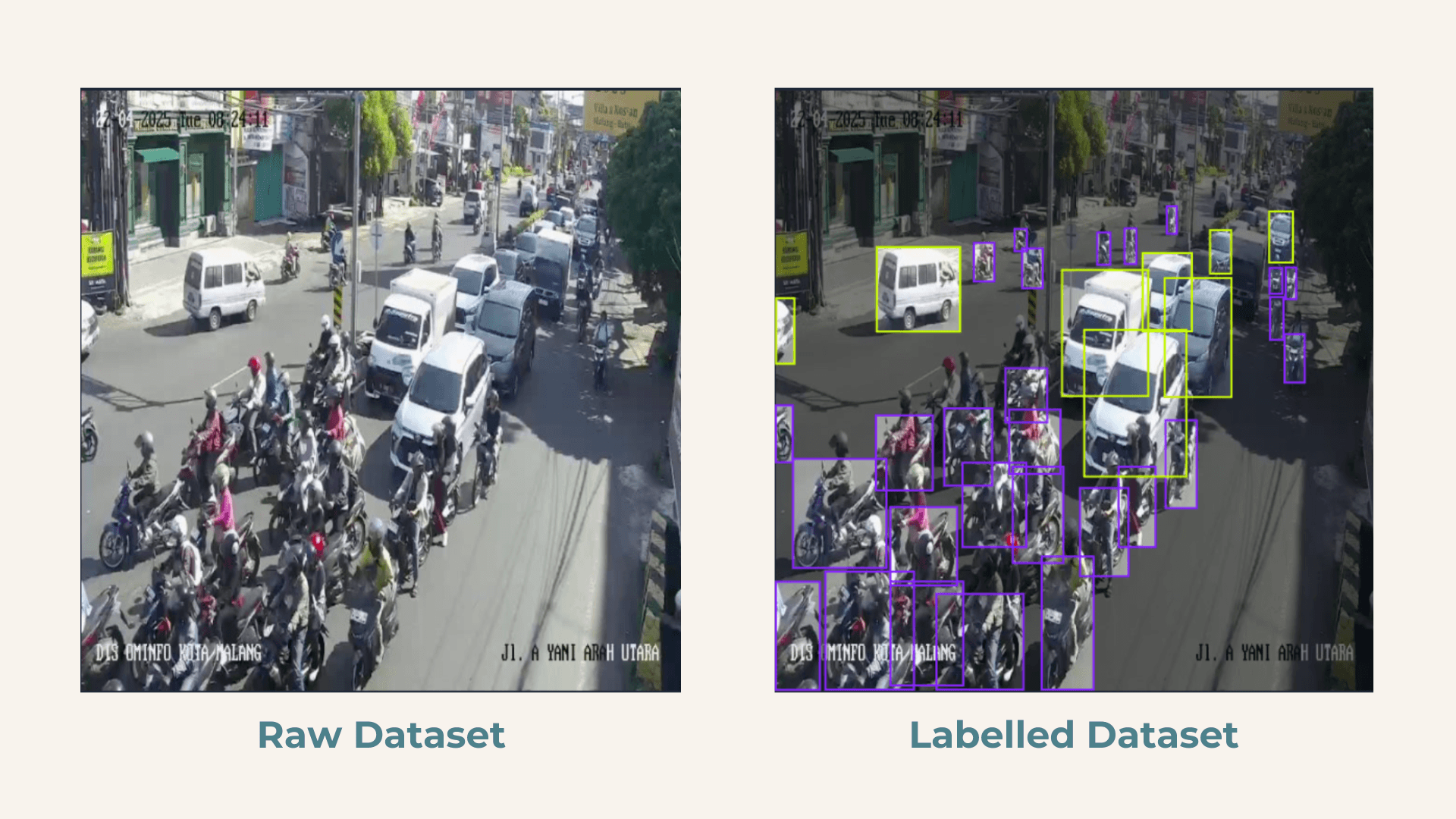
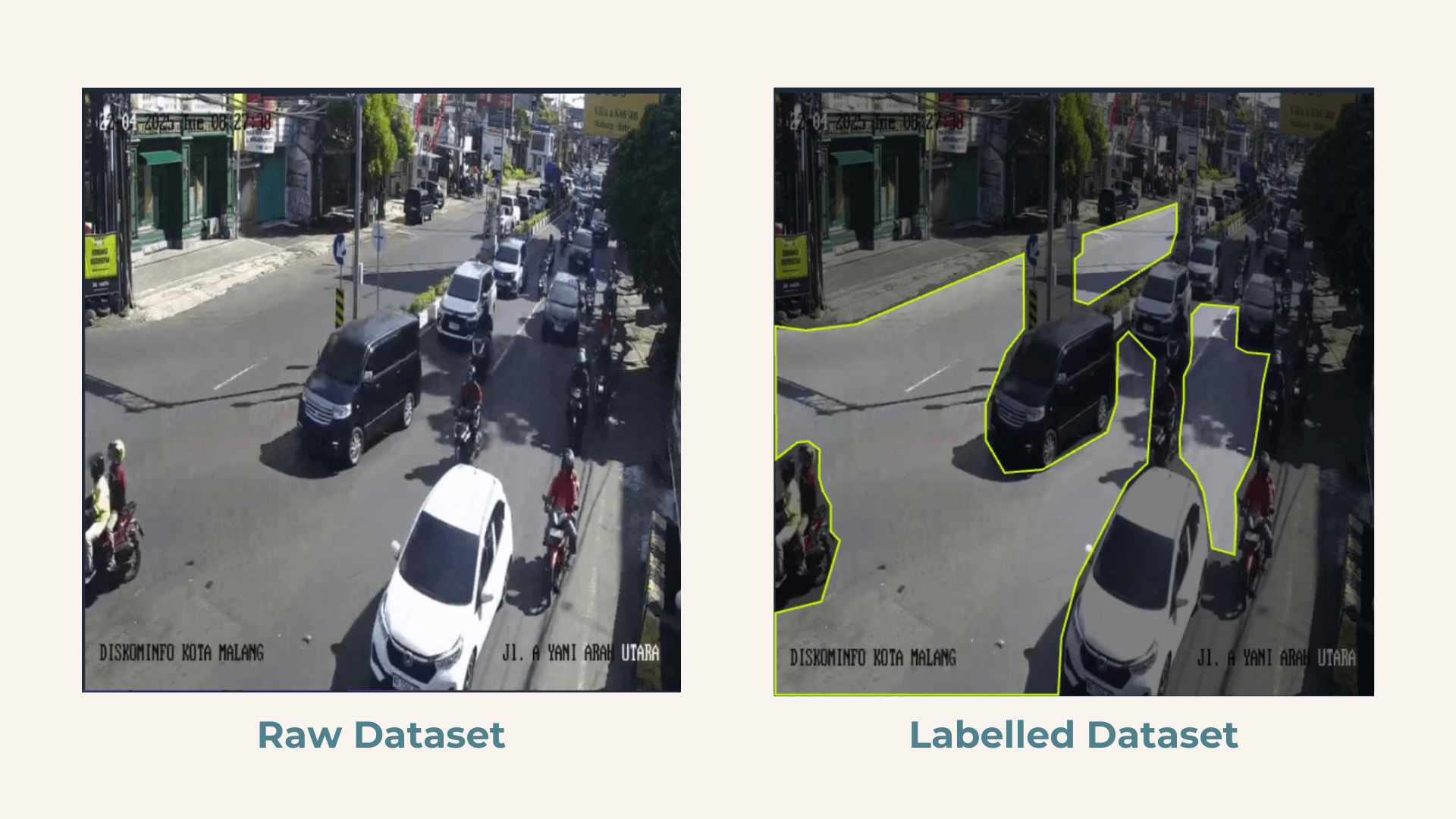
ARCHITECTURE
Two branches of a single frame meet again at the feature vector: the detector says what and how many, the segmenter says out of how much road, and the motion between frames says how fast. Only then does anything classify.
How each model was trained
The same shape ran three times — YOLO11n for detection, YOLO11n-seg for segmentation, and the classifiers over the extracted features. Only the dataset and the metrics change; the SVM adds a grid search over its hyperparameters in the training step.
Speed is measured using Lucas-Kanade sparse optical flow — tracking the pixel displacement of detected vehicle centroids frame-to-frame and converting it to a normalised speed feature. Combined with SSIM-based frame sampling to skip visually redundant frames, this keeps the pipeline at 18–22 FPS on real CCTV footage.
RESULTS
Vehicle detection — YOLO11n
| Class | P | R | mAP@50 | mAP@50-95 |
|---|---|---|---|---|
| All | 0.853 | 0.831 | 0.908 | 0.682 |
| Car | 0.862 | 0.907 | 0.952 | 0.799 |
| Motorbike | 0.844 | 0.754 | 0.864 | 0.564 |
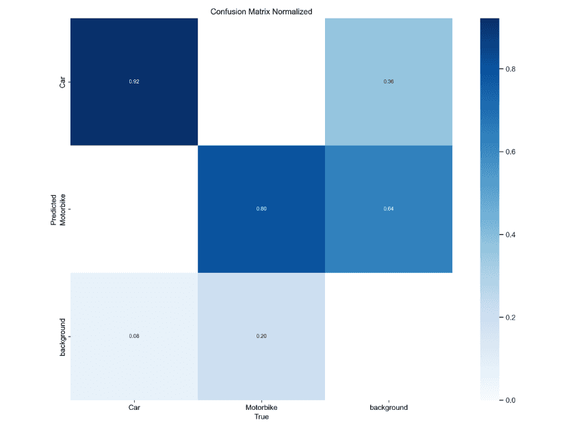
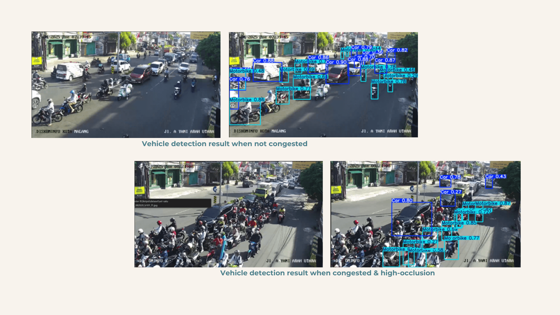
Cars are close to solved at 95.2% mAP@50. Motorbikes are the honest number: 75.4% recall, and mAP@50-95 of 56.4%. They are small, they cluster, and in a queue they physically occlude one another — which is exactly the condition the system is meant to detect.
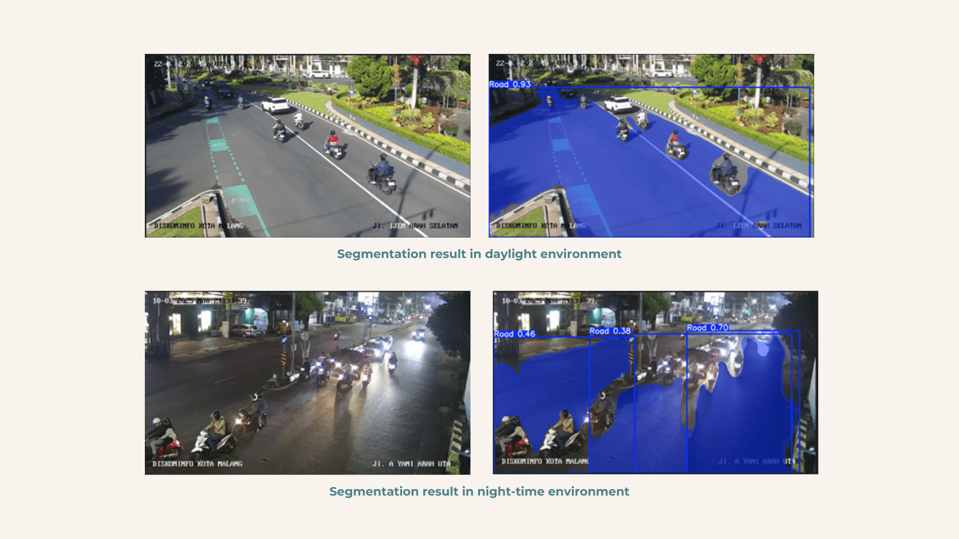
Road segmentation — YOLO11n-seg
Decent in daylight and clearly the weaker half of the pipeline at night: glare and uneven street lighting break the road mask into fragments, and everything computed against road area degrades with it.
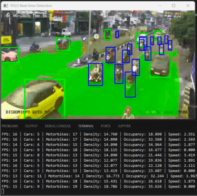
Feature extraction
The raw YOLO outputs — boxes and masks — are converted per frame into the six numerical features, printed alongside the overlay while the stream runs. This is the layer that made the dataset: 20,113 rows of real traffic state.
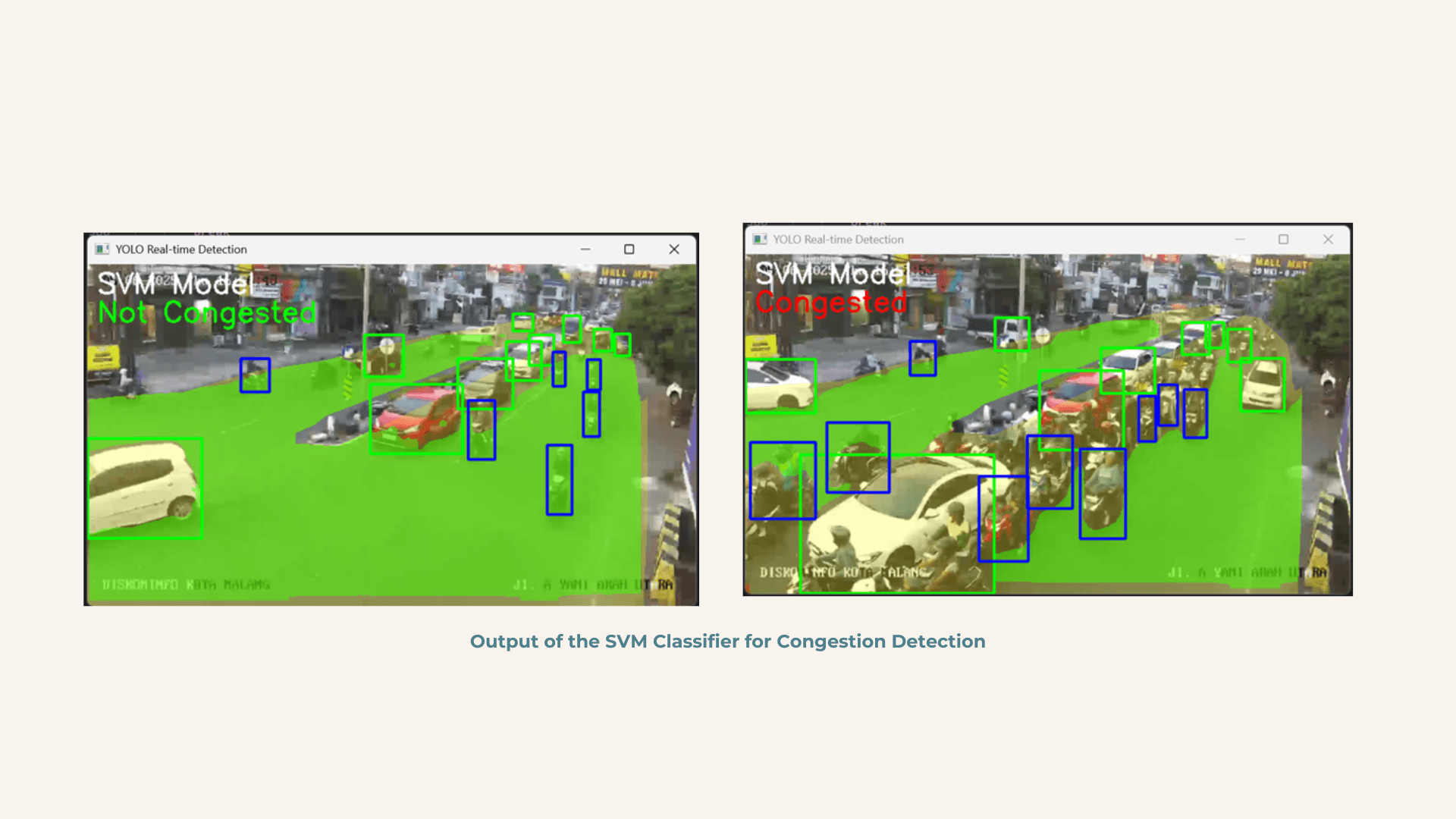
The classifier — two of them
| Model | Accuracy | Precision | Recall | F1 |
|---|---|---|---|---|
| Neural network | 97.54% | 98% | 98% | 98% |
| SVM · grid-searched | 97.38% | 98.2% | 96.5% | 97.35% |
Both were trained on the same 20,113 rows and both land within two-tenths of a percent of each other, which says more about the features than about either model. The neural network is the one the conclusion runs on.
TrafficClassifier(
  (layer_1):     Linear(in_features=6, out_features=64, bias=True)
  (relu1):       ReLU()
  (dropout1):    Dropout(p=0.3, inplace=False)
  (layer_2):     Linear(in_features=64, out_features=32, bias=True)
  (relu2):       ReLU()
  (dropout2):    Dropout(p=0.3, inplace=False)
  (output_layer):Linear(in_features=32, out_features=1, bias=True)
  (sigmoid):     Sigmoid()
)
Six inputs, two hidden layers of 64 and 32 units, ReLU with 0.3 dropout on each, one sigmoid output. Small on purpose — the features carry the signal, so the model doesn't have to.
WHAT'S WEAK
Two numbers in the results are worse than the headline, and both were in the defence rather than hidden behind it.
And a scope limit worth stating plainly: every number here is measured on Malang City CCTV. The thesis makes no claim about other cities, other camera heights, or other traffic mixes.
STACK
- Python
- YOLO11
- PyTorch
- OpenCV
- Lucas-Kanade flow
- scikit-learn · SVM
- SSIM sampling
- Roboflow
TIMELINE
- OCT — DEC 2024 · PROPOSAL
Literature review, problem scoping and proposal document — establishing the four-feature hypothesis and choosing YOLO11 as the detector.
- JAN 2025 · PROPOSAL DEFENCE
Proposal defended and approved at Petra Christian University.
- JAN — MAY 2025 · BUILD
Dataset sampling and labelling in Roboflow (850 detection frames, 430 segmentation frames), fine-tuning both YOLO11n models, extracting 20,113 feature rows, and training the NN and SVM classifiers.
- JUN 2025 · THESIS DEFENCE
Full pipeline — detection, segmentation, Lucas-Kanade speed, classification — running live at 18–22 FPS. 97.5% accuracy on the unseen test set.
LESSON
The feature engineering beat the bigger model. Counting vehicles is the obvious signal and the wrong one — twenty moving and twenty stopped are the same count. Once flow, density, occupancy and speed were right, two hidden layers were enough to separate them, and a grid-searched SVM landed within two-tenths of a percent of the network. The work was never in the classifier.